F-statistic Calculation: Exploring its Role in Machine and Deep Learning

xPetersue

Aug 21, 2023 • 5 min read

Linear regression, a cornerstone of statistical modeling, has the remarkable ability to reveal intricate relationships hidden within data. It's the compass that guides us through the labyrinth of variables, guiding us to better predictions and deeper insights. But how do we assess the strength and significance of a regression model? Enter the F-statistic, a familiar metric in the world of linear regression, which scrutinizes the overall performance of our models. Yet, beneath the surface of the F-statistic lies a more profound revelation: a fundamental equation that unveils the intricate dance between predictors and variance. In this journey, we'll traverse the landscape of linear regression, starting with the familiar territory of the F-statistic and venturing into the heart of variance decomposition.

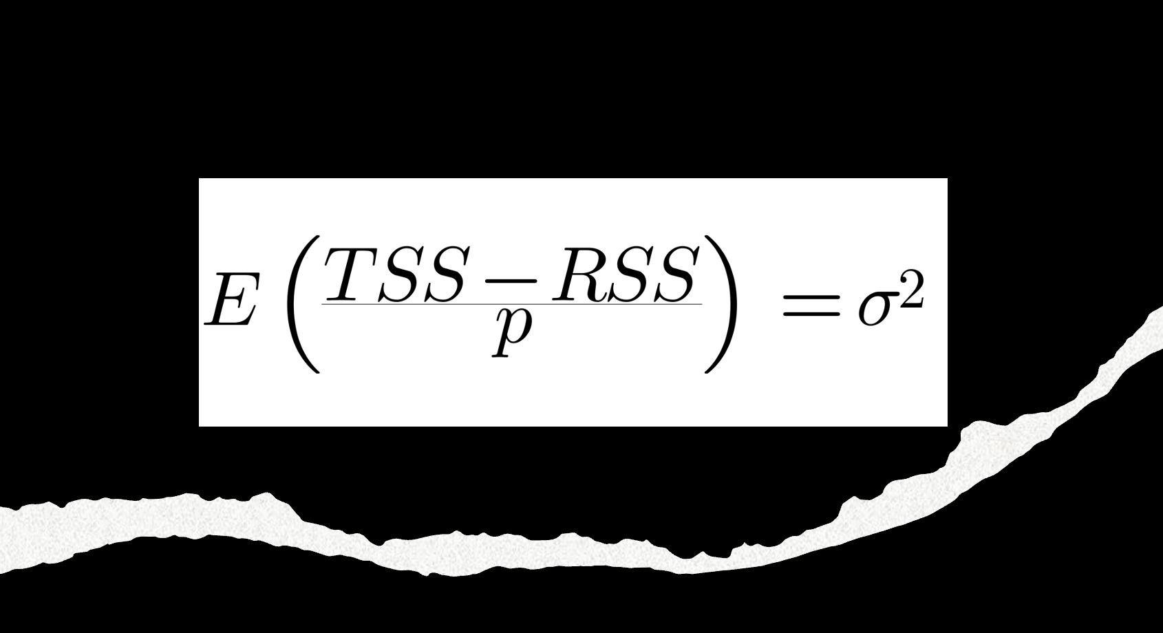
Here, we'll encounter the equation E{(TSS - RSS)/p} = σ^2, a powerful tool that enables data scientists to decode the secrets hidden within their data.

Let's first delve into the concept of the five components:

E{...} represents the expected value, which is a way to find the average or mean of a random variable. In the context of linear regression, it's often used to calculate the expected value of a particular expression or statistic.
TSS (Total Sum of Squares) measures the total variability in the dependent variable (the one you're trying to predict) Y. It is calculated as the sum of the squared differences between each observed Y value and the overall mean of Y, or rather it defined as:TSS = Σ(Yi - Ŷ)^2, where Yi is an observed Y value, and Ŷ is the mean of all Y values.

RSS (Residual Sum of Squares) measures the variability that is not explained by your regression model. It is calculated as the sum of the squared differences between the observed Y values and the predicted Y values (the values predicted by your regression model), or rather it's defined as:RSS = Σ(Yi - Ŷi)^2, where Yi is an observed Y value, and Ŷi is the predicted Y value from the model.

Note:

Equation A is a more general formula that can be applied to various predictive modelling scenarios where you have observed and predicted values based on any modelling approach (not limited to linear regression).

Equation B is specific to linear regression and focuses on quantifying the unexplained variability in the dependent variable by the linear regression model. It helps assess the goodness of fit of the linear regression model to the data.

p represents the number of predictors or independent variables in your linear regression model. These are the variables that you use to predict the dependent variable Y.
σ^2 (Sigma squared) represents the variance of the error term in your linear regression model. The error term (ε) represents the difference between the observed Y values and the predicted Y values. σ^2 is the variance of these errors and is often referred to as the "error variance."

Here is the explanation of the entire formula:

E{(TSS - RSS)/p} = σ^2

(TSS - RSS)/p

This part divides the difference between TSS and RSS by the number of predictors (p). This is essentially finding the average reduction in variability in Y that your model provides per predictor. It's a measure of how much each predictor contributes to explaining the variability in Y.

E{(TSS - RSS)/p}

In this context, you're finding the average or expected value of the average reduction in variability across different samples of data. The expectation is taken over various possible samples, and it represents the average behavior of this expression over those samples.

σ^2(Sigma squared)

The formula equates this expected value to the error variance (σ^2). This implies that if your linear regression model is a good fit for the data, then the average reduction in variability per predictor should equal the error variance. In other words, your predictors are explaining the same amount of variability as the error term, which is what you expect in a good model.

To conclude: this formula is to assess the goodness of fit of your linear regression model by comparing how much it reduces the variability in the dependent variable compared to the error variance, on average, per predictor. If the formula holds true, it suggests that your model is doing a good job of explaining the variability in the data.

How is this equation employed in machine learning and deep learning?

The equation E{(TSS - RSS)/p} = σ^2 and the concepts related to variance decomposition are not typically used directly in machine learning and deep learning in the same way they are used in traditional linear regression.

Instead, these concepts have evolved into other techniques and methods that serve similar purposes. Here's how the fundamental idea of understanding the contribution of predictors to variance reduction is applied in machine learning and deep learning.

Let's use the equation E{(TSS - RSS)/p} = σ^2 to explain the concepts of variance decomposition, feature importance, and variable selection in the context of a linear regression model predicting home prices.

Example: Predicting Home Prices with Linear Regression

Suppose you're a data scientist working for a real estate agency, and your task is to build a linear regression model to predict home prices. You have a dataset with various predictors, including square footage, number of bedrooms, neighborhood, and year built. Here's how you can apply the equation and related concepts:

1. Variance Decomposition:

First, you fit a linear regression model to predict home prices using all available predictors (features).
You calculate the total sum of squares (TSS), which measures the total variance in home prices based on the actual data points.
You calculate the residual sum of squares (RSS), which quantifies the unexplained variance in home prices by the regression model.

Now, you can use the equation:

E{(TSS - RSS)/p} = σ^2

TSS−RSS represents the reduction in total variance explained by the model.
p is the number of predictors in the model.
σ^2 is the error variance, representing the unexplained variability in home prices.

Interpretation: The equation tells you that, on average, each predictor (feature) in your model contributes an amount equal to σ^2 to the reduction in the total variance of home prices for your dataset. This quantifies the average contribution of each predictor to the reduction in variance.

2. Feature Importance:

Next, you want to assess the importance of each feature in predicting home prices. To do this, you examine the coefficients (weights) assigned to each predictor by the linear regression model.

For example:

Square Footage Coefficient: 0.5
Number of Bedrooms Coefficient: 0.3
Neighborhood Coefficient: 0.2
Year Built Coefficient: 0.1

Interpretation: The coefficients represent the change in the predicted home price for a one-unit change in each feature while holding other variables constant. A larger coefficient suggests a stronger impact on the predicted price. In this case, square footage has the most substantial influence, followed by the number of bedrooms, neighborhood, and year built.

3. Variable Selection:

You aim to simplify your model while retaining predictive accuracy. To do this, you consider removing less important features.
Based on the feature importance (coefficients) and the equation's insight, you decide to keep the top three predictors: square footage, number of bedrooms, and neighborhood.

By retaining these influential features, you simplify the model while still capturing the primary drivers of home prices.

In summary, the equation E{(TSS - RSS)/p} = σ^2 provides a theoretical foundation for understanding how each predictor contributes to the reduction in variance in a linear regression model. This understanding can guide feature selection, helping you identify the most important features and simplify your model while maintaining predictive accuracy.

Sign up for more like this.